Python (SymPy) Programming for Fourier analysis

This article deals with the Fourier expansions using SymPy, a Python library for symbolic calculations. An example in this article provides an identity for pi, which will be examined numerically by Numpy, a Python library for numerical calculations. An introductory collection of SymPy usage can be found in the previous article:

pianofisica.hatenablog.com

Orthogonality of trigonometric functions
Fourier series expansions
Example

Orthogonality of trigonometric functions

The following set of functions

$\qquad\displaystyle{\frac{1}{\sqrt{2\pi}},~\frac{\cos x}{\sqrt{\pi}},~\frac{\cos 2x}{\sqrt{\pi}},~\frac{\cos 3x}{\sqrt{\pi}},\, \dots,~\frac{\sin x}{\sqrt{\pi}},~\frac{\sin 2x}{\sqrt{\pi}},~\frac{\sin 3x}{\sqrt{\pi}},\,\dots}$

provides an orthonormal basis for functions defined on a region $-\pi\leq x\leq \pi$ . One can check it by running the following code on Python:

import sympy as sp

x = sp.symbols('x')
def c(m, x): 
   if m == 0: return 1/sp.sqrt(2*sp.pi)
   else: return sp.cos(m*x)/sp.sqrt(sp.pi)
def s(m, x): return sp.sin(m*x)/sp.sqrt(sp.pi)

def cc(m,n): return sp.integrate(c(m,x)*c(n,x), (x, -sp.pi, sp.pi))
def cs(m,n): return sp.integrate(c(m,x)*s(n,x), (x, -sp.pi, sp.pi))
def ss(m,n): return sp.integrate(s(m,x)*s(n,x), (x, -sp.pi, sp.pi))

Then, for example

CC = [[],[],[],[],[]]
for m in range(5):
  for n in range(5):
    CC[m].append(cc(m,n))
print(CC)

shows (for $m,n=\{0,1,2,3,4\}$ )

$\qquad\displaystyle{\int^\pi_{-\pi} dx \frac{\cos mx}{\sqrt{\pi}} \frac{\cos nx}{\sqrt{\pi}}=\delta_{m,n} }$

SIimilarly

SS = [[],[],[],[],[]]
for m in range(5):
  for n in range(5):
    SS[m].append(ss(m,n))
print(SS)

shows (for $m,n=\{0,1,2,3,4\}$ )

$\qquad\displaystyle{\int^\pi_{-\pi} dx \frac{\sin mx}{\sqrt{\pi}} \frac{\sin nx}{\sqrt{\pi}}=\delta_{m,n} }$

and finally

CS = [[],[],[],[],[]]
for m in range(5):
  for n in range(5):
    CS[m].append(cs(m,n))
print(CS)

shows

$\qquad\displaystyle{\int^\pi_{-\pi} dx \frac{\sin mx}{\sqrt{\pi}} \frac{\cos nx}{\sqrt{\pi}}=0}$

Thus one may be able to convince yourself that the orthonormality of the set of functions.

Fourier series expansions

A series expansion of a function $f(x)$ defined on a region $-\pi\leq x\leq \pi$ given in the following form

$\qquad \displaystyle{\begin{aligned}f(x)&=A_0\frac{1}{\sqrt{2\pi}}+A_1\frac{\cos x}{\sqrt{\pi}}+B_1\frac{\sin x}{\sqrt{\pi}}+A_2\frac{\cos 2x}{\sqrt{\pi}}+B_2\frac{\sin 2x}{\sqrt{\pi}}+\dots\\ &=A_0\frac{1}{\sqrt{2\pi}}+\sum_{n=1}^\infty \left(A_n\frac{\cos nx}{\sqrt{\pi}}+B_n\frac{\sin nx}{\sqrt{\pi}}\right)\end{aligned}}$

is called Fourier expansion of $f(x)$ . Owing to the orthonormality of the functions, the coefficients are determined by

$\qquad \displaystyle{A_0=\int^\pi_{-\pi} dx \, \frac{1}{\sqrt{2\pi}} \, f(x),\quad A_n=\int^\pi_{-\pi} dx \, \frac{\cos nx}{\sqrt{\pi}} \,f(x), \quad B_n=\int^\pi_{-\pi} dx \, \frac{\sin nx}{\sqrt{\pi}}\, f(x)}$

Example

f(x)=x

$\qquad \displaystyle{f(x)=x \quad (-\pi\leq x\leq \pi)}$

sp.init_printing()
def f(x): return x
def a(n): return sp.integrate(c(n,x)*f(x), (x, -sp.pi, sp.pi))
def b(n): return sp.integrate(s(n,x)*f(x), (x, -sp.pi, sp.pi))
A = []
B = []
for n in range(10):
  A.append(a(n))
  B.append(b(n))
[A,B]

gives

$\qquad\displaystyle{A_0=0, \quad A_n=0, \quad B_n=(-1)^{n+1}\sqrt{\pi}\,\frac{2}{n} \qquad (n\geq1)}$

thus its Fourier expansion is given by

$\qquad\displaystyle{x=2\left\{\frac{\sin x}{1}-\frac{\sin 2x}{2}+\frac{\sin 3x}{3}-\frac{\sin 4x}{4}+\dots\right\}}$

Built-in: fourier_series

While SymPy has a built-in command for obtaining Fourier coefficients:

ff = sp.fourier_series(f(x), (x, -sp.pi, sp.pi)).truncate(8)  
# truncate( ) specifies how many order to expand
ff

Drawing a graph

To visualize how much extent the expansion approximates the function, let it draw the graphs of expansion truncated $\ n=1,3,7$ :

import matplotlib.pyplot as plt
import numpy as np

D = 50
xmin = -np.pi
xmax = np.pi

def Ff(n, x):
   return sp.fourier_series(f(x), (x, -sp.pi, sp.pi)).truncate(n)  
p = np.linspace( xmin, xmax, D)
def FF(n,k): return float(Ff(n, x).subs(x, p[k]))
Q1 = []
Q3 = []
Q7 = []
for k in range(D):
   Q1.append(FF(1,k))
   Q3.append(FF(3,k))
   Q7.append(FF(7,k))
q = p
q1 = np.array(Q1)
q3 = np.array(Q3)
q7 = np.array(Q7)

plt.plot(p ,q)
plt.plot(p ,q1)
plt.plot(p ,q3)
plt.plot(p ,q7)
plt.show()

provides

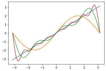
where blue line is for the original function, and orange, green and red, are accordingly truncations at order $\ n=1,3,7$ , including higher modes.

Pi (Leibniz/Euler's series)

The Fourier expansion obtained above implies, by setting $x=\pi/2$ , the following identity:

$\qquad\displaystyle{\frac{\pi}{4}=1-\frac{1}{3}+\frac{1}{5}-\frac{1}{7}+\dots}$

This series is referred to as Leibniz's series or Euler's series. Examining this series numerically shall be done by running the following code:

k = sp.var('k', integer = True)
def p(n): return 4+4*sp.summation((-1)**k/(2*k+1), (k, 1, n))

gives a finite sum of the series till $n$ -th term. For example, 1,000 terms gives

float(p(1000))

$\qquad 3.14259165\dots$

while the actual value is

float(sp.pi)

$\qquad \pi=3.141592653589793\dots$

Then one finds that 1,000＝ $10^3$ terms reproduce it 3-digit accuracy.

10,000 terms

float(p(10000))

$\qquad 3.14169264\dots$

improves it 1-digit, but it takes computer resources and takes some time to evaluate.

Using a list gives a faster computation:

N = 10000
P = [4]
def q(k): return 4*(-1)**k/(2*k+1) + P[k-1]
for k in range(1,N):
  P.append(q(k))
P[N-1]

for $10^{7}$

N = 10**7
P = [4]
def q(k): return 4*(-1)**k/(2*k+1) + P[k-1]
for k in range(1,N):
  P.append(q(k))
P[N-1]

gives

$\qquad 3.14159255\dots$

so that the accuracy seems improved by inclusions of more terms.

Keywords: Python, SymPy, Fourier series, Orthonormal functions